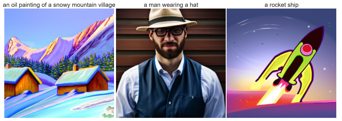
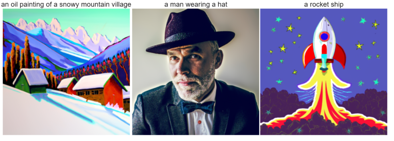
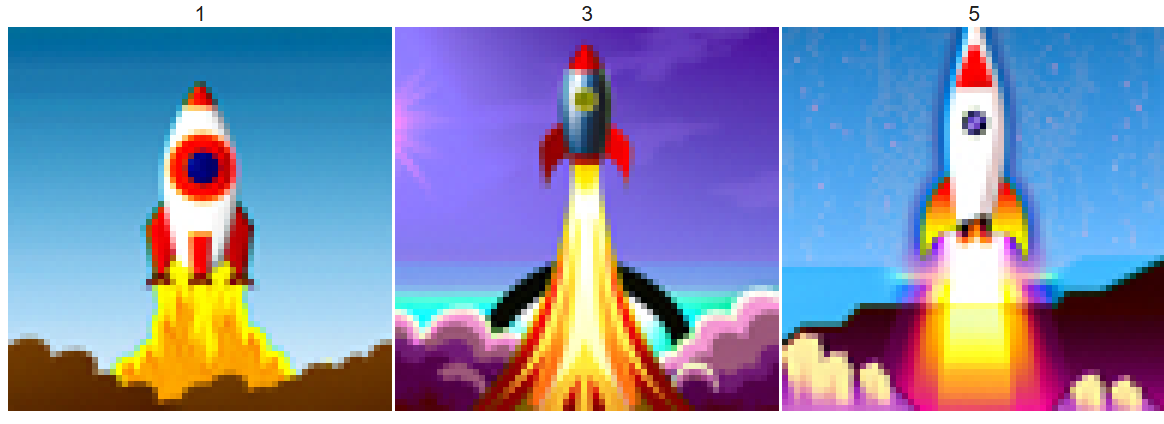
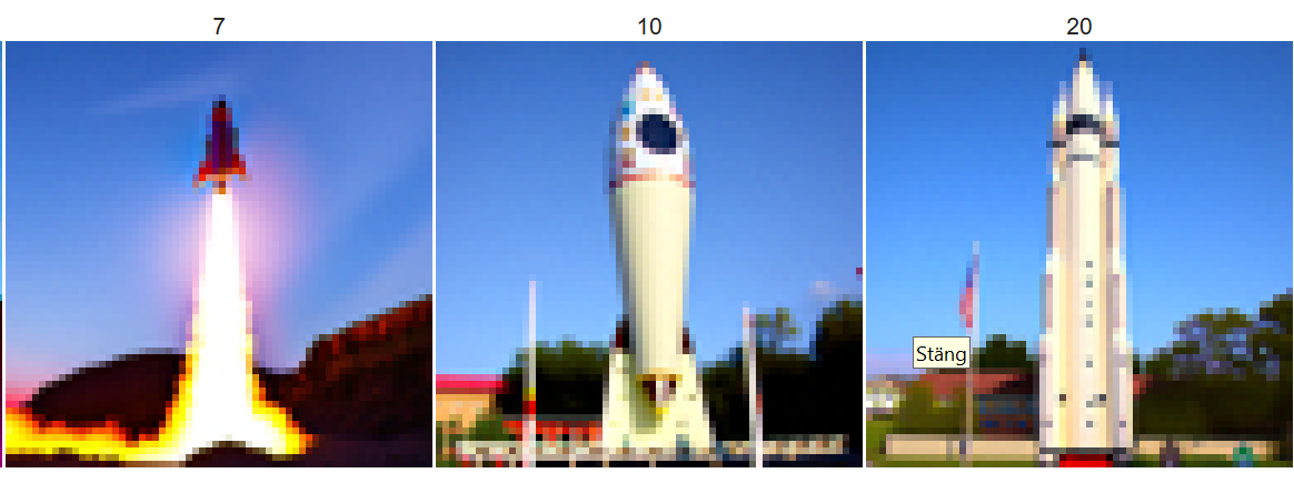
For this part, we set up the diffusion model with a random seed (185). This seed will be used throughout the project. In part A, we work with images of size 64x64 pixels, which might not be as sharp. In part B, the images improve significantly. Below, we show results with different inference steps.


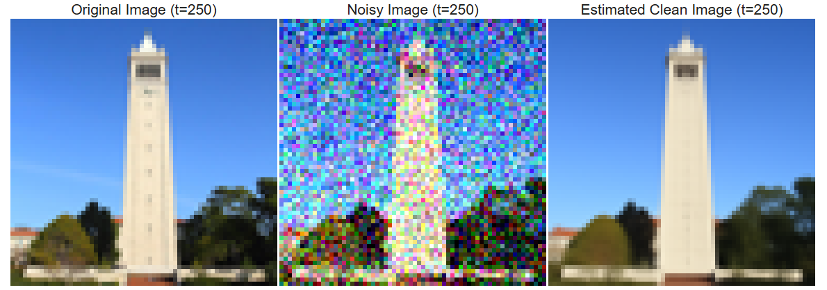
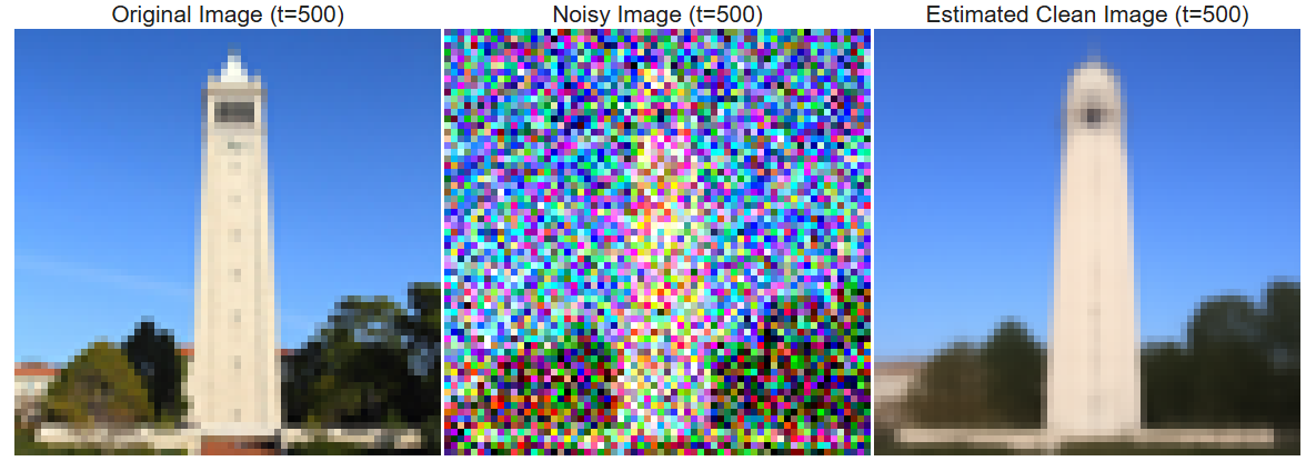
Adding noise progressively to an image is key in the diffusion process. This allows the model to learn how to reverse noise, recovering the clean image. Below are examples of the test image at various noise levels:


Gaussian blurring was used to denoise the images. This method is not effective, as seen below:


A U-Net estimates and removes Gaussian noise. The model considers the timestep as an input parameter, making it easier to determine the amount of noise to remove:
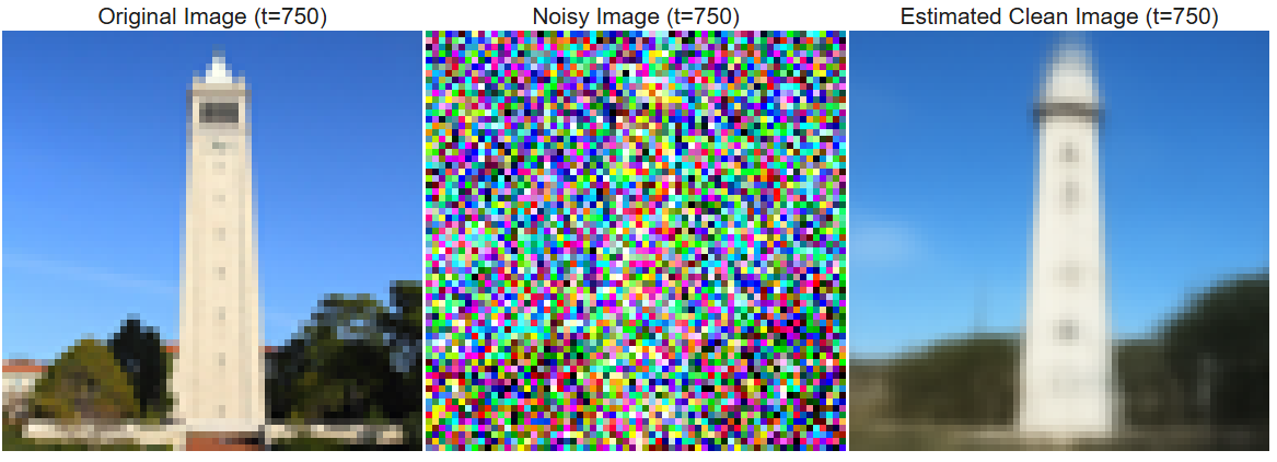
Iterative denoising works better than classical methods. To speed up the process, denoising is performed every 30 timesteps. Below is the progression of denoising and the final comparison to classical methods:
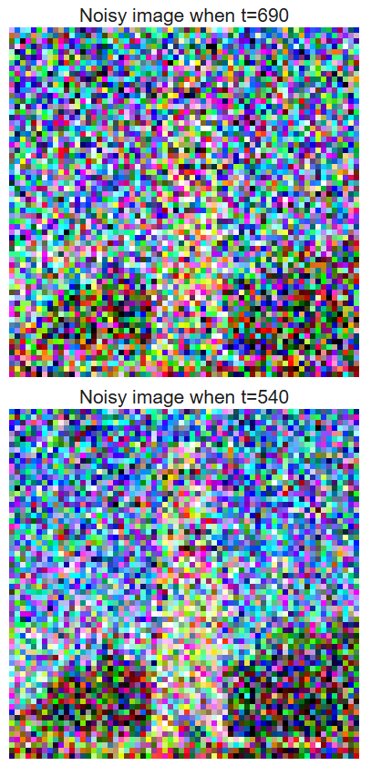
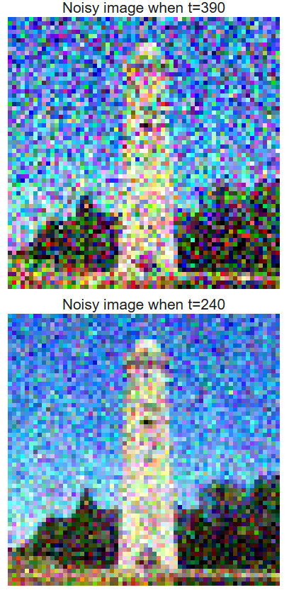
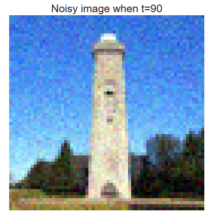

In this part, we used the trained diffusion model to generate five random images. These images were sampled starting from pure noise and progressively denoised to create realistic outputs. This demonstrates the model's ability to synthesize diverse images based on the learned data distribution.

To improve the quality of generated images, we implemented Classifier-Free Guidance (CFG). This technique combines a conditional noise estimate based on a text prompt with an unconditional noise estimate, weighted by a guidance parameter γ. The new noise estimate is computed as:
ϵ = ϵu + γ(ϵc − ϵu)
By setting γ > 1, we achieve significantly higher-quality images at the expense of diversity. For γ = 0, the model generates unconditional results, and for γ = 1, it creates conditional results. The images below demonstrate the improvement in quality using CFG with γ = 7.

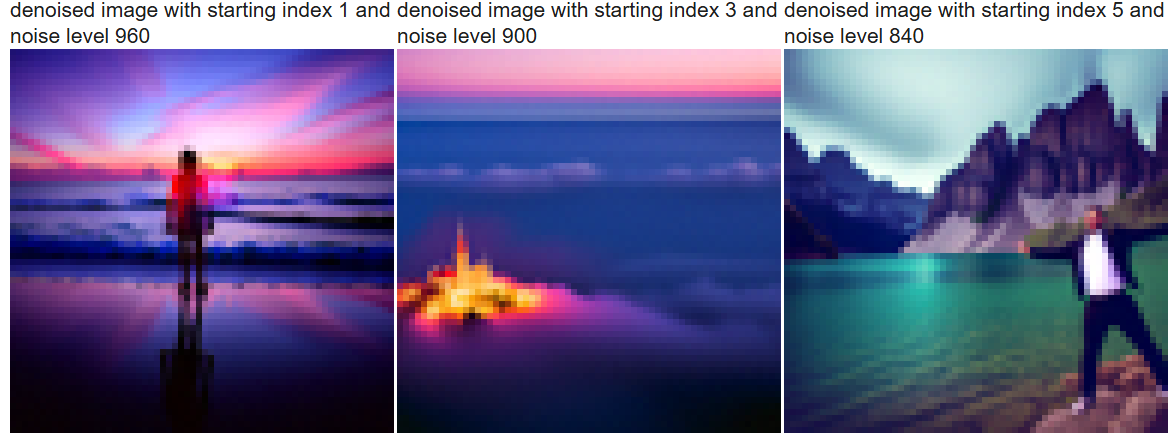
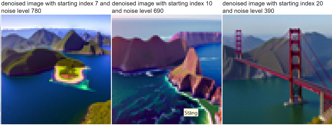
In this part, we explored the SDEdit algorithm to make creative edits to an image. By adding noise to a real image and denoising it using the diffusion model, we force the noisy image back onto the manifold of natural images. The extent of the edit depends on the noise level—higher noise levels lead to larger edits, while lower noise levels retain more of the original structure.
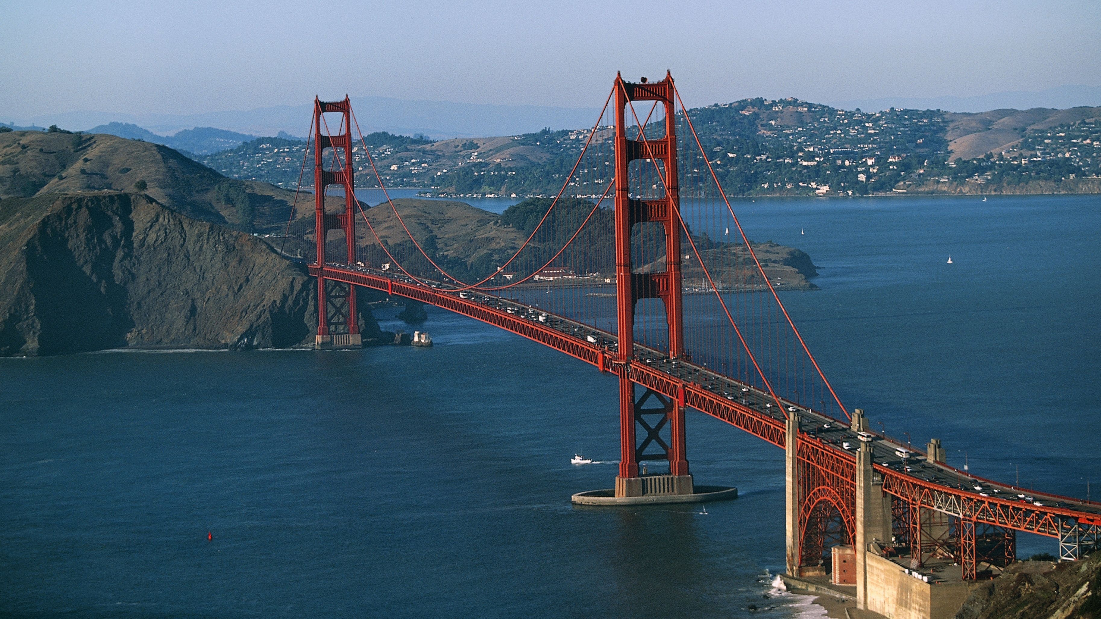
Using the prompt "a high quality photo", we applied this technique to the original test image at noise levels [1, 3, 5, 7, 10, 20]. The results demonstrate how the image transitions from noisy to more refined, with creative edits made by the model.
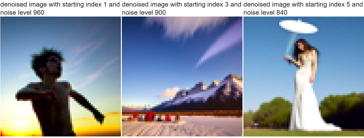
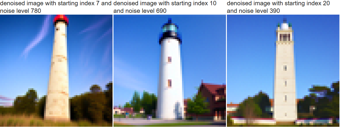
We repeated the process on two additional test images using the same noise levels. Below are the results for one of the custom images.
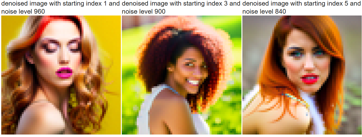
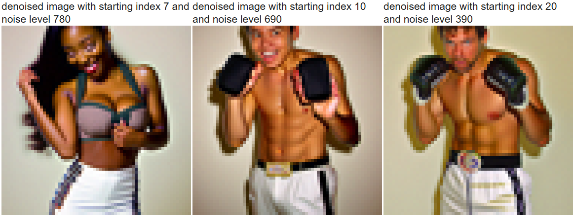
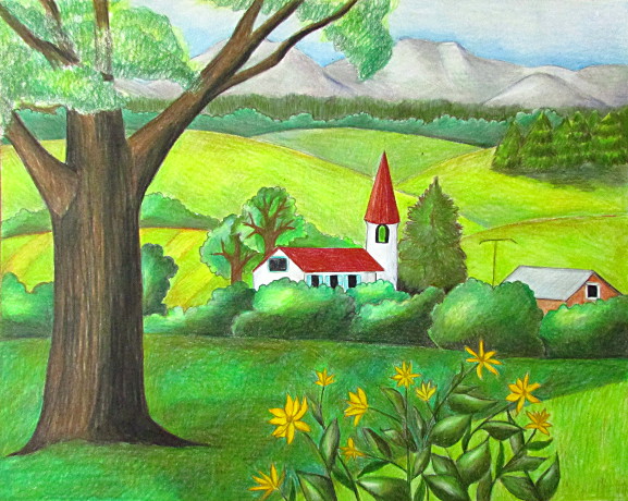
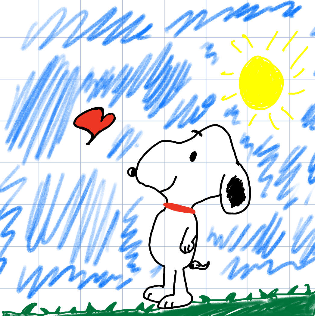
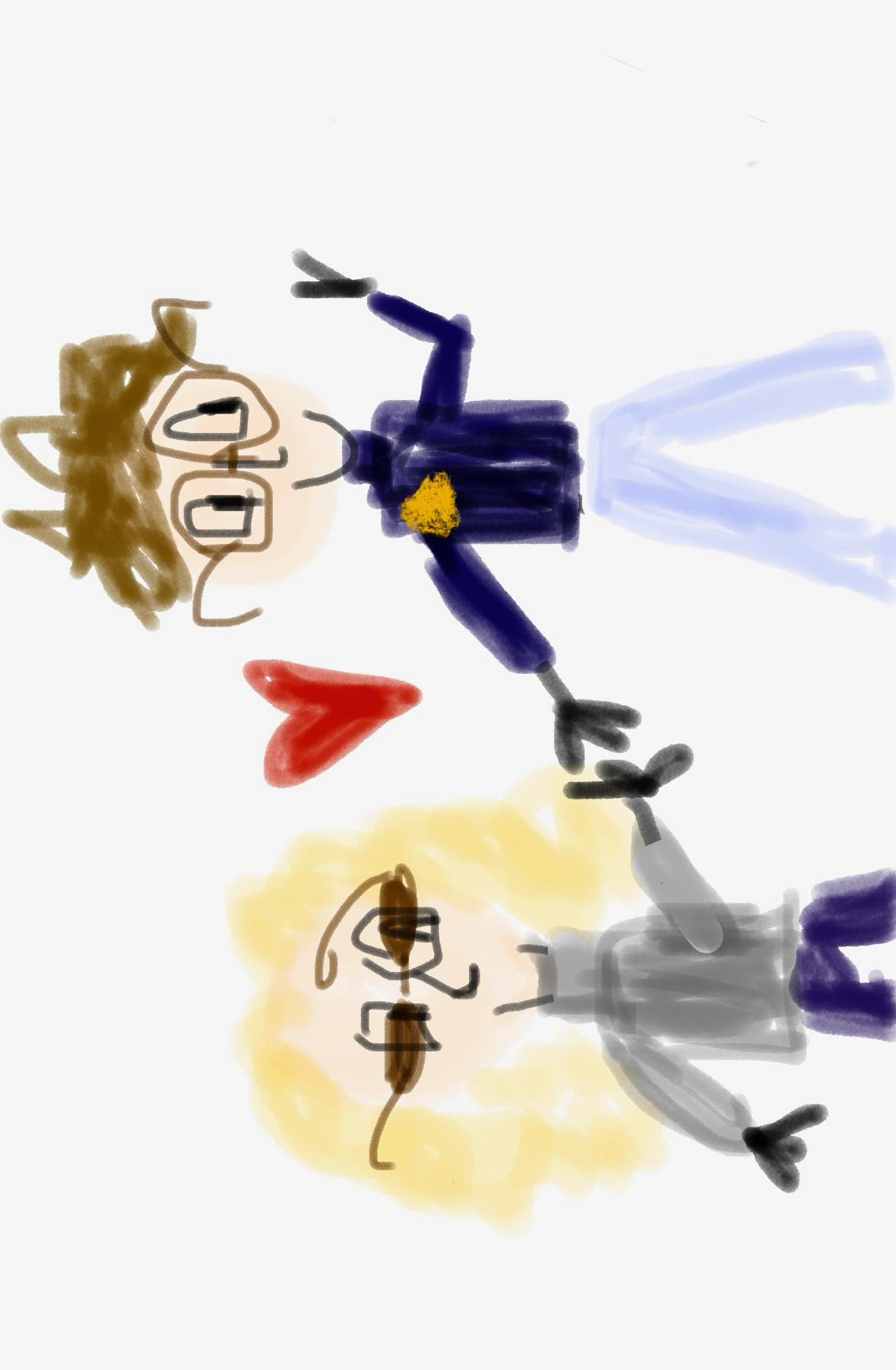
In this part, we apply the same image-to-image translation technique but use hand-drawn images as input. Below is one hand-drawn image from the web and two images drawn by me.



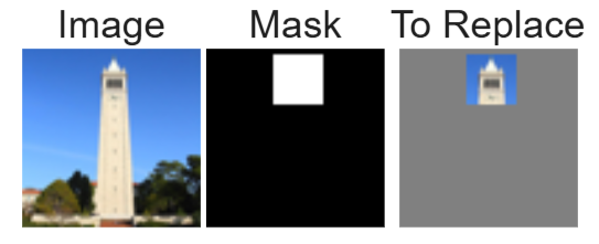
In this section, we explore inpainting by following a method inspired by the RePaint paper. Given an image (xorig) and a binary mask (m), we create a new image that preserves the original content where the mask is 0 and introduces new content where the mask is 1.
To achieve this, we use the diffusion denoising loop with a small modification. At each denoising step, after obtaining xt, we force it to retain the original pixels where m is 0, effectively leaving the masked areas intact. The process is defined as:
xt ← m * xt + (1 − m) * forward(xorig, t)
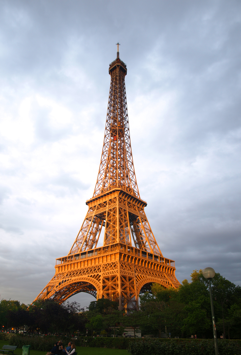
By iteratively applying this approach, the diffusion model fills in the masked area with new content while preserving the rest of the image. We applied this technique to inpaint the top of the Campanile using a custom mask.

We further experimented with inpainting on two custom images, using different masks to replace selected areas of each image.

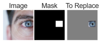

In this part, we perform image-to-image translation with guidance from a text prompt. By combining the model's inpainting ability with language control, we can adjust the output to match a specific description. This goes beyond simple "projection to the natural image manifold" by incorporating semantic information from the prompt.
To achieve this, we modify the prompt from "a high quality photo" to a descriptive phrase, applying different noise levels [1, 3, 5, 7, 10, 20]. The resulting images should maintain characteristics of the original image while aligning with the text prompt.
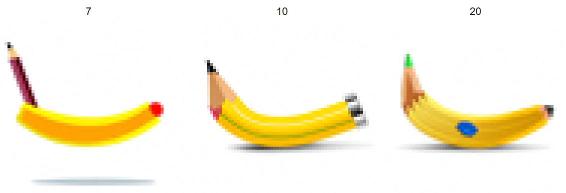
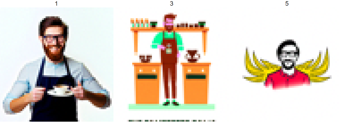
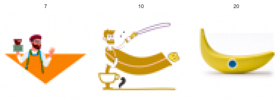
We applied the same process to two custom images using the prompt "a photo of a hipster barrista" and "a pencil" and varying noise levels. The outputs show a blend of the original image (a banana) and the characteristics described in the prompt.

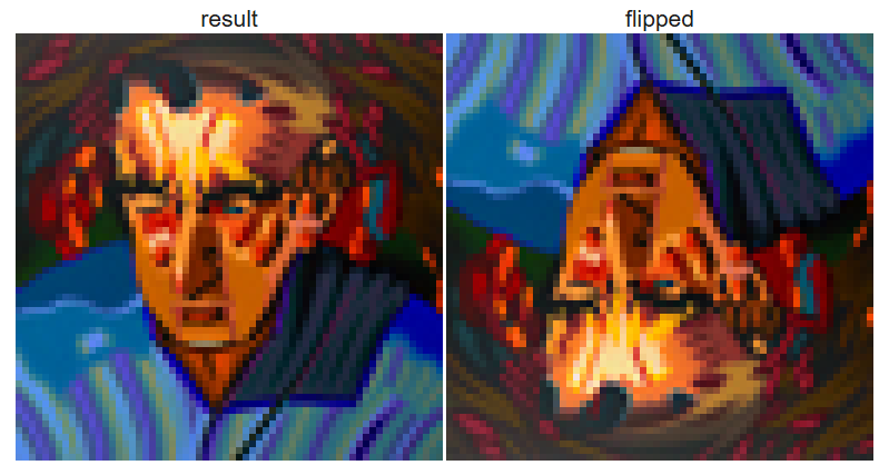
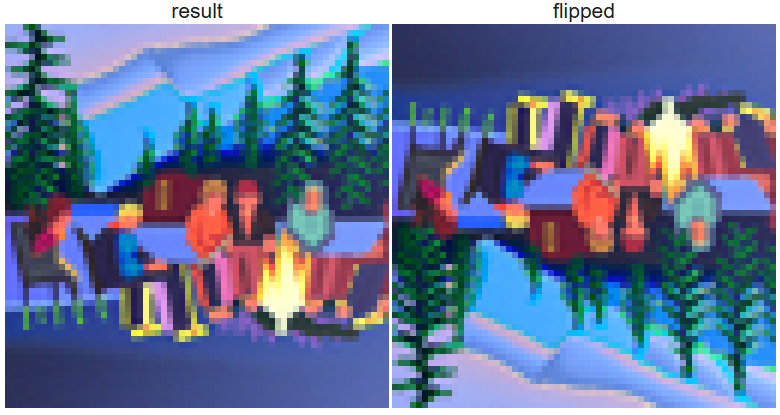
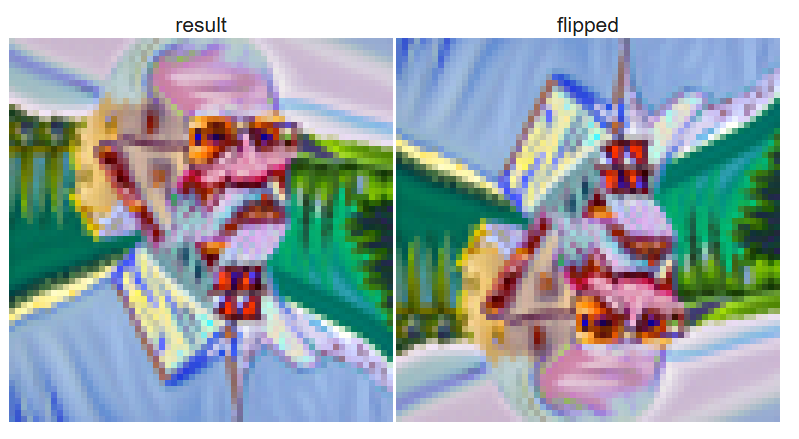
In this part, we use diffusion models to create visual anagrams—images that show two different scenes when viewed upright and flipped upside down. Our goal is to create an image that appears as "an oil painting of an old man" when viewed normally, and as "an oil painting of people around a campfire" when flipped.
To achieve this effect, we perform diffusion denoising on an image xt at a particular timestep t, with two different prompts. First, we denoise the image using the prompt "an oil painting of an old man", obtaining a noise estimate ϵ1. Next, we flip xt upside down and denoise it with the prompt "an oil painting of people around a campfire", resulting in ϵ2. We then flip ϵ2 back to its original orientation and average it with ϵ1 to create the final noise estimate ϵ.
The steps for creating a visual anagram are as follows:
ϵ1 = UNet(xt, t, p1) using the prompt "an oil painting of an old man".xt upside down and generate ϵ2 = flip(UNet(flip(xt), t, p2)) using the prompt "an oil painting of people around a campfire".ϵ = (ϵ1 + ϵ2) / 2.ϵ to obtain the final image.Below are examples of visual anagrams created using this method. The first image appears as "an oil painting of an old man" when viewed normally and as "an oil painting of people around a campfire" when flipped. We also include two additional anagram illusions that reveal different images when flipped upside down.
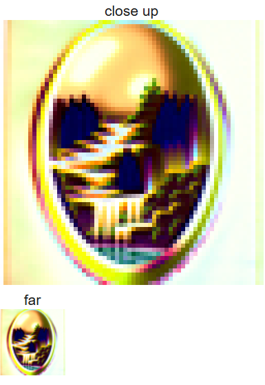
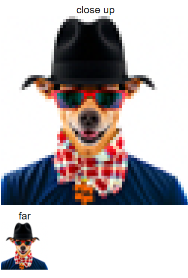
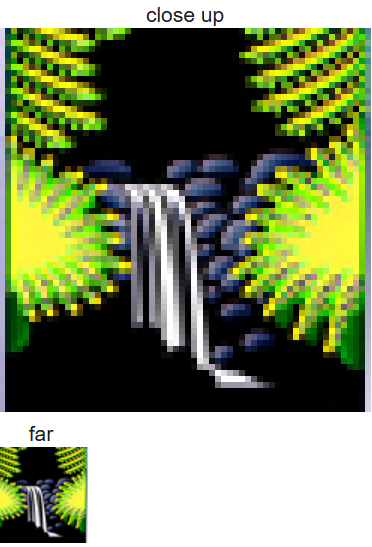
In this part, we implement Factorized Diffusion to create hybrid images, inspired by techniques from project 2. A hybrid image combines different elements that appear as one thing when viewed from a distance and something else up close. Here, we use a diffusion model to blend low and high frequencies from two different text prompts, creating a composite effect.
The process involves estimating noise using two prompts, combining the low frequencies from one estimate and the high frequencies from the other. This approach allows us to create an image that looks like one subject from afar and transforms into a different subject upon closer inspection.
The steps for generating a hybrid image are as follows:
ϵ1 = UNet(xt, t, p1), with the first prompt.ϵ2 = UNet(xt, t, p2), with the second prompt.ϵ1 and a high-pass filter to ϵ2: ϵ = flowpass(ϵ1) + fhighpass(ϵ2).
ϵ to complete a reverse diffusion step and obtain the final hybrid image.For this part, we use a Gaussian blur with a kernel size of 33 and sigma of 2 for the low-pass filter, which smooths out the details in the first noise estimate, while the high-pass filter captures the finer details from the second estimate.
Below are examples of hybrid images created with this technique. The first image appears as a skull from afar and as a waterfall up close. We also include two additional hybrid illusions that transform depending on viewing distance.
I thought this first part of the project was really cool. I think it is very intersting how the images are generated and can't wait for part B which I assume will be even cooler.
To start, we train a simple denoiser Dθ that maps a noisy image xnoisy to a clean image xclean. The L2 loss is optimized as:
ℒ = ||Dθ(xnoisy) - xclean||²
We use a UNet for the denoiser. It consists of downsampling and upsampling blocks with skip connections, capturing both global and local features. This structure is ideal for image-to-image tasks like denoising.
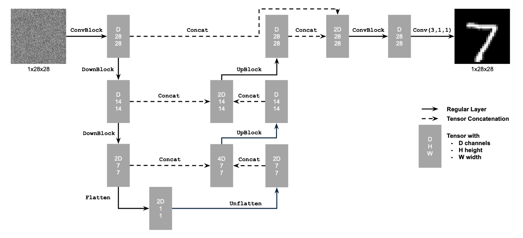
In this part, we implement and visualize the noising process for generating training data. The objective is to train a denoiser Dθ to map noisy images xnoisy to clean images xclean, minimizing the L2 loss:
ℒ = ||Dθ(xnoisy) - xclean||²
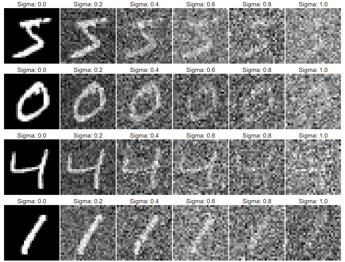
To achieve this, clean MNIST digits xclean are progressively noised to create training pairs (xnoisy, xclean).
Below is the output of the implemented noising process applied to a normalized MNIST digit. The images show the effect of increasing noise levels:
For training we used the image class pairs. I used a batchsize of 256, 5 epochs, sigma = 0.5 and the Adam Optimizer with a learning rate of 1e-4. Below you can find the loss during training.
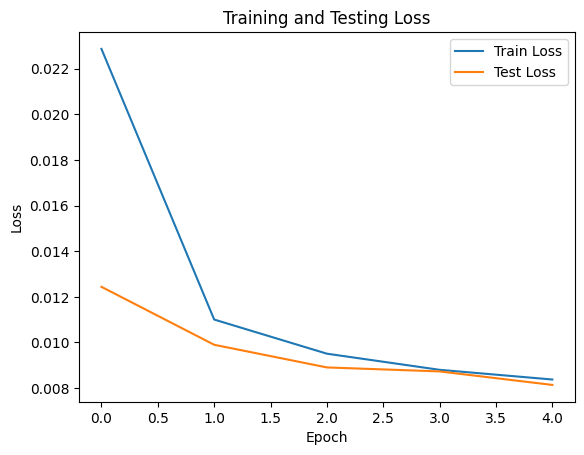
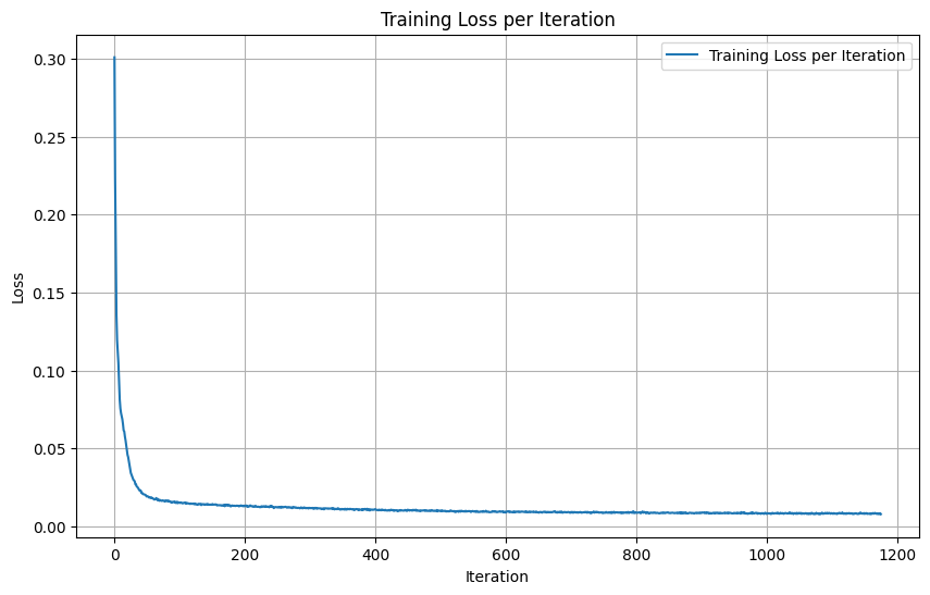
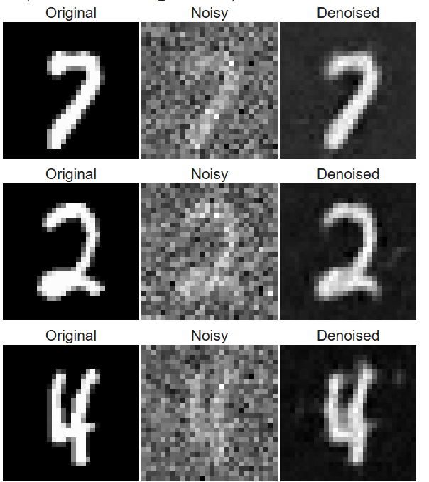
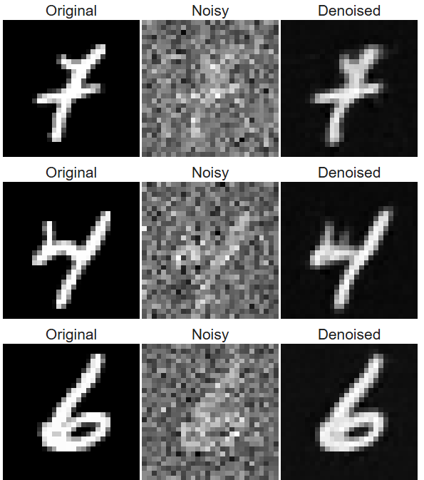
The results from the training can be seen below, where I show the performance after 1 epoch and after 5 epochs. As you can see the model becomes much better after 5 epochs.
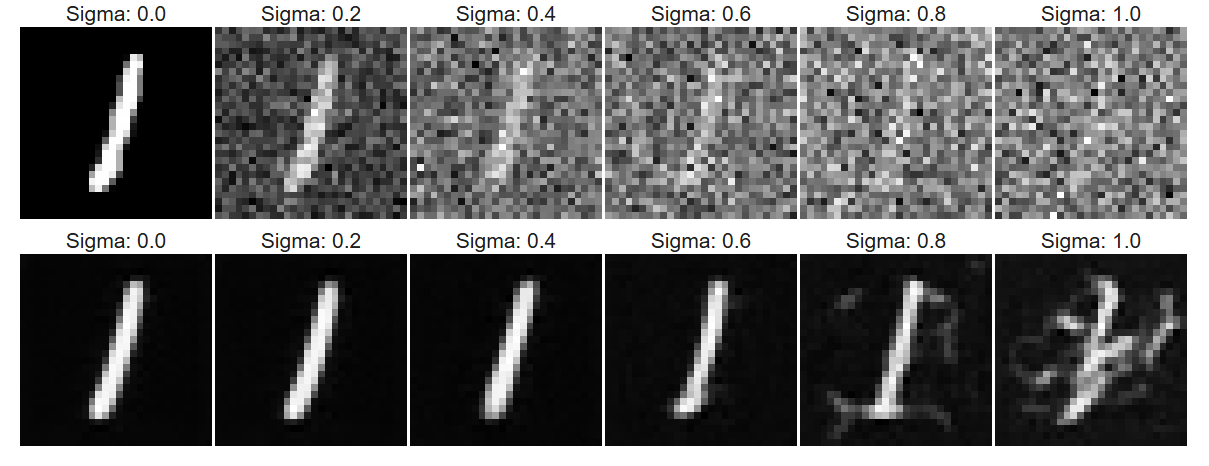
The model was as stated trained using a sigma value of 0.5. But it is intersting to see how well it can perform with higher versus lower values for sigma i.e more and less noise than during training. In the image below you can see that performance.
Previously, our UNet model predicted the clean image. In this section, we update the approach to predict the noise ϵ added to the image instead. This allows us to start with pure noise ϵ ∼ N(0, I) and iteratively denoise to generate a realistic image x.
Instead of implementing time conditioning first and then adding class conditioning, we simultaneously condition the UNet on both the timestep t and the class of the digit. Using the equation:
xt = √ᾱtx0 + √(1−ᾱt)ϵ, ϵ∼N(0,1)
we generate a noisy image xt from x0 for a timestep t∈{0,1,…,T}. When t=0, xt is clean, and when t=T, xt is pure noise. For intermediate values of t, xt is a linear combination of the clean image and noise. The derivations for β, αt, and ᾱt follow the DDPM paper, and we set T=400 due to the simplicity of our dataset.
To handle time conditioning, we integrate fully connected layers to embed t into the UNet. For class conditioning, we use a one-hot vector to represent each digit class ({0,…,9}). We further add two fully connected layers to embed the class vector.
Below is the updated UNet architecture, which includes both time and class conditioning as well as the new training algorithm used:
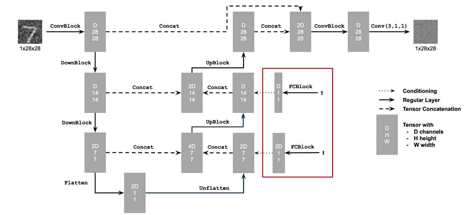
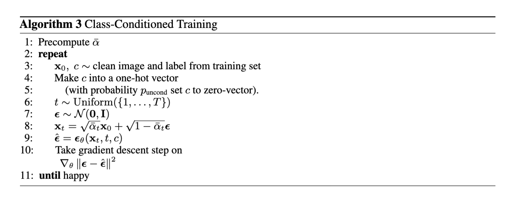
The training process involves generating noisy images xt for random timesteps, computing their one-hot class vectors, and training the UNet to predict ϵ. The addition of class conditioning ensures better control over the generated images, while time conditioning enables iterative denoising. As we can see
in the results presented below after the twentieth epoch the model works very well and produces fine, correct and detailed numbers.
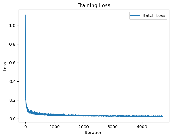


If we now only look at the Time Conditioned UNet, i.e no classes. The results are presented below. As we can see the numbers are not as good without the classifier free guidance.
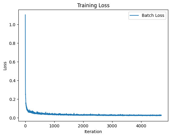


Very cool and fun project. The most interting part was definetely to see how adding classes (CFG) increased the performance of our model and how easy teh change was to do.