
For the first we are supposed to fit a Neural Field to a an image. This is done by creating a Multi Layer Perecptron with Sinusoidal Positional Encoding. The architecture of the MLP is presented below.

As you can see in the image above, the MLP has 3 layers with each having 256 hidden dimensions. All of the hidden layers uses the ReLU activation function and the final output layer using the Sigmoid activation function instead. Throughout part 1 I used the Adam optimizer function and Mean Squared Error as loss. For this part I tried out some different settings for the hyper parameters to see what worked best. Below you will se the results.


Below I present the PSNR (Peak Signal to Noise Ratio) and Loss plots which we used as the metrics to evaluate the performance of our model.
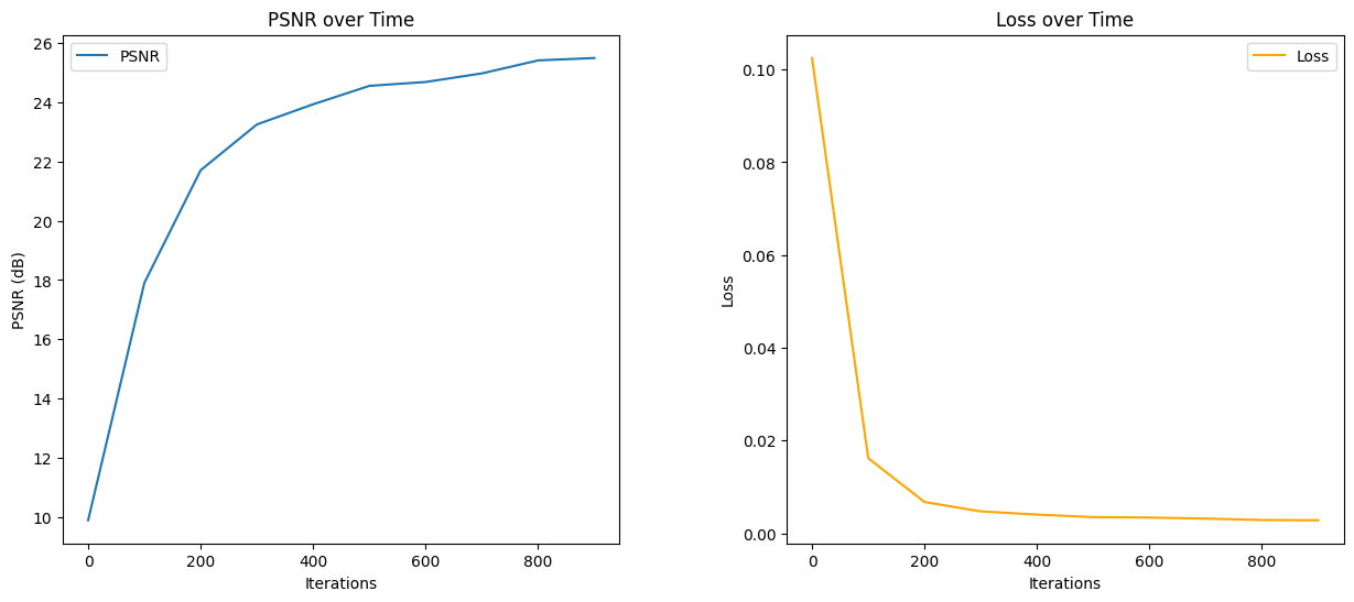
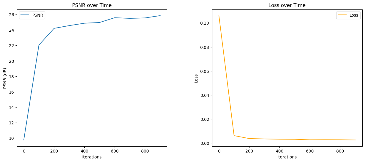

As we can see the model which has 10 positional encoding function works great for both learning rates and number of iterations. The model converges faster with a higher learning rate but ultimately reaches the same PSNR. However if we increase the number of positional encodings the model does not work well with reproducing the image, however the PSNR is still high.
I also tested the model on an image of Ali the famous boxer. This image had fewer pixels than the image of the fox, making it easier for the model to get a good results. As we can see below the results are in fact better.

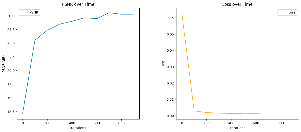
Training took around 40 seconds using the GPU however since the model almost converged after 500 iterations we could decrease training time to around 20 seconds which I consider very fast
To create the dataset, we start with a list of images, camera-to-world matrices, and the focal length, from which we compute the intrinsic matrix. The intrinsic matrix is essential as it encodes the camera's internal parameters, such as focal length and principal point offset, enabling accurate projection of 2D pixels into 3D rays within the scene.
For each ray, we randomly select a pixel from the available images. This pixel, combined with its corresponding camera parameters, is projected into 3D space as a ray originating from the camera's position. These sampled rays simulate the viewing experience of a camera moving through the scene and allow the model to learn from a wide range of perspectives. Random sampling also introduces stochasticity, which helps prevent overfitting by exposing the model to diverse ray configurations during training.
This ray sampling process ensures that the neural radiance field captures the spatial relationships and color information necessary to synthesize accurate novel views. Below is a visualization illustrating the ray sampling process from some of the cameras; showing all of them would make the representation too cluttered and unclear.
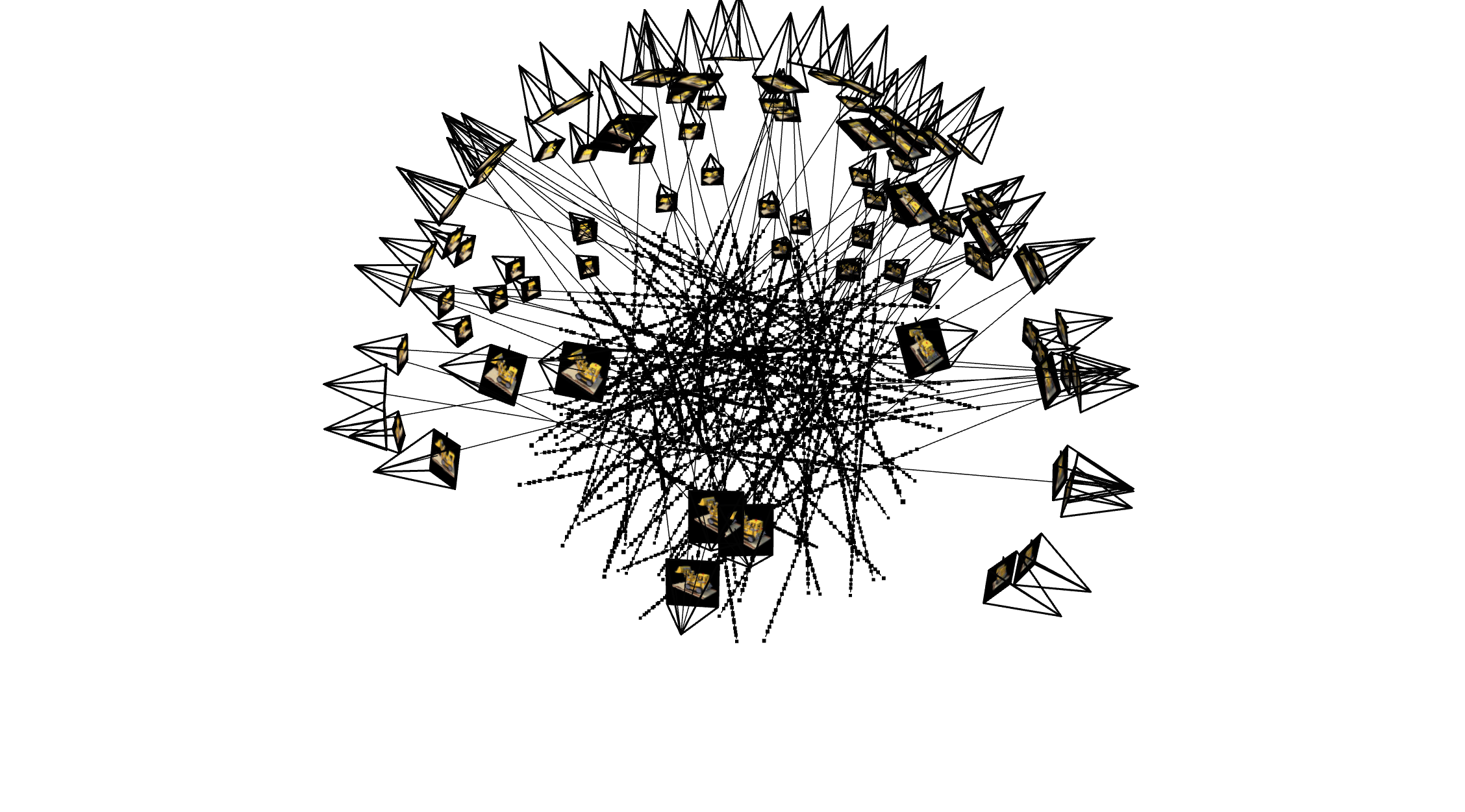
Using the sampled rays, we perform discrete steps along each ray in 3D space. At each step, a small perturbation is applied to the sampling positions to improve robustness. This randomization ensures that the model does not overfit to a fixed sampling pattern and enhances its ability to generalize. At these discrete points, we query the neural radiance field to predict the RGB color and density (opacity) values.
The outputs are aggregated using the volume rendering equation, which integrates the contributions of each point along the ray. The equation combines the radiance at each point with the density and transmittance (how much light passes through previous points) to create a realistic rendering of the scene. This approach allows for accurate modeling of lighting, shading, and occlusion effects.
When training the network I did it over 3000 iterations with a batchsize of 10000. Again we use the Adam optimizer and MSE as loss function. Now we have a larger MLP for which the architecture is presented in the image below.

The novel views generated by NeRF are synthesized by rendering the scene from viewpoints not present in the training dataset. However, these views are often of lower quality due to limited information from the original dataset. Sparse or uneven camera coverage reduces the model's ability to infer unseen regions, leading to artifacts or blurring in these areas. Occluded regions (those not visible in any input image) are especially challenging, as the model must rely entirely on learned priors.
The outputs are aggregated using the volume rendering equation:

Below is a visualization of the progress during training, highlighting the iterative improvement of both standard and novel views.
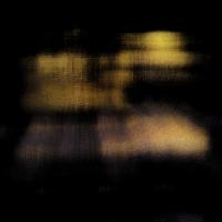
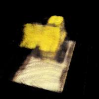
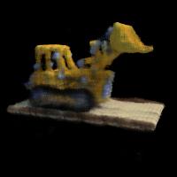
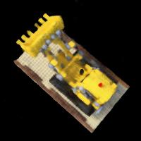
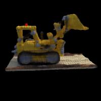
And below you can see how the reconstruction from same novel view became better during training, notice how already after 600 iterations it is pretty good and after 2700 it is really good:
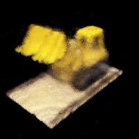
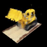
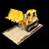

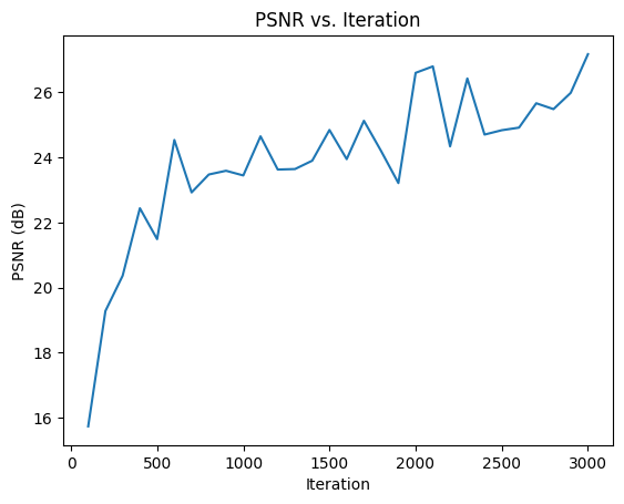
I trained the model for around 10-15 minutes which made the model reach a Peak Signal to Noise Ratio of around 27 which I thought was good enough for the short training duration. However if I would increase the number of iterations and batchsize I could probably increase the quality of the final 3D which was created using all the newly created novel views. Below is the PSNR plot for the training of the nerf. As you can see in the image the model has not yet converged which means by increasing the number of iterations would in fact yield an even better result
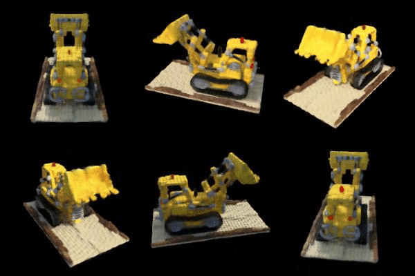
The final 3D model constructed is presented in the GIF below
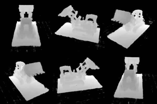
Since NeRFs output both RGB values and density (or opacity), we can leverage this to achieve something fascinating: depth rendering. Instead of generating RGB values, we can modify the output to represent a single value between 0 and 1, indicating how far each pixel is from the camera.
All and all a very fun project where I learnt a lot. I thought it was very interesting using NeRFs not only rendered surfaces but actually cool 3D stuff.